This is an old revision of the document!
Table of Contents
ADMB Framework : Synthetic Data
Here we describe how synthetic data is generated, which is useful when testing various models and admb code.
The Model
The ADMB framework is first tested on synthetic data. In the first step, we start with a simple model, which is the same (simple) model used for real data:
| Ni,t | = | (Ni,t-1-Ci,t-1)e-M | [1] |
|---|---|---|---|
| f(Ni,0,qk,s,M) | = | -(2s2)-1[ln(Ii,t,k)-ln(qkNi,t)]2-ln(s) | [2] |
We generate synthetic data using parameters in Table 1. Next, we attempt to recover the parameters using the objective function defined in [2]
Table 1: Data model parameters
| Parameter | Description | Dimension |
|---|---|---|
| Ni,0 | Recruitment for cohort i | m-by-1 |
| M | Natural mortality | Scalar |
| Ci,t | Catch of indivduals in cohort i, at age t | m-by-(maxage+1) |
| Ii,t,k | Survey index for cohort i, at age t, by survey k | At most m-by-(maxage+1)-by-num_surveys |
| s | Standard deviation for I | Scalar |
| qk | Catchability of survey k | 1-by-num_surveys |
Assumptions
The number of cohorts m, Ni,0, the number of surveys, the catchabilities qk, s and M are input by the user. The catch is randomly generated (see formula below), and the survey indices are generated to comply with the model's statistical assumption that:
Implementation and Coding
Data can be generated using the following code:

CC(i-1,j) = rand(1,1) * cfactor/n * N(i-1,j);
…should probably be changed to be independent of n and have less variance.
- generate_data.m
function N = generate_data(N0,q,s,M, filename, cohorts, years, surveys, requested_observations,year_offset,in_cfactor);
% filegenerator(N0,q,s,M, filename, cohorts, years, surveys, observations, year_offset, cfactor)
%
% Generates .dat file for cod problem.
%
% VERSION WITH SIMPLE MODEL - no random effects, and just one M!
%
% Written by Lennart Frimannslund

if (exist('year_offset','var')==0 | length(year_offset) == 0),
  year_offset = 1980;
end;

% Generate filename if not specified
if (exist('filename','var') == 0 | length(filename) == 0),
  c = clock;
  filename = sprintf('herring-%s-%02d.%02d.%02d',date,c(4),c(5), ...
                     floor(c(6)));
  clear c;
end;


% Get number of surveys
if (exist('q','var') ~= 0 & length(q) ~= 0),
  surveys = length(q);
end;

% s - Generate random number between 0 and 1
if (exist('s','var') == 0 | length(s) == 0),
  s = rand;
end;

% M - Generate random number between 0 and 0.2
if (exist('M','var') == 0 | length(M) == 0),
  M = rand(1,1) * 0.2;
end;


% If no of cohorts not specified - generate random number between 1 and 6
if (exist('cohorts','var') == 0 | length(cohorts) == 0),
  cohorts = ceil((rand*5)) + 1;
end;

% years - if not specified, generate random number between 5 and 25
if (exist('years','var') == 0 | length(years) == 0),
  years = ceil((rand*20)) + 5;
end;

% surveys - if not specified, generate random number between 1 and 6
if (exist('surveys','var') == 0 | length(surveys) == 0),
  surveys = ceil((rand*5)) + 1;
end;

% if not specified - generate which fraction of maximum possible
% observations available
%if (exist('observations','var') == 0 | length(observations) == 0),
%  observations = ceil(rand * surveys * years * cohorts);
%end;


% Define N0 if not supplied
% exp(N0) between 0 and 3
%if (exist('N0','var') == 0 | length(N0) == 0),
%  N0 = 3 * rand(1,1);
%end;

% Generate q - between 0.1 and 0.8
if (exist('q','var') == 0 | length(q) == 0),
  q = 0.7 * rand(1,surveys) + 0.1;
end;


% Input variables now in place - generate data set itself
%
% For the most part translated line-by-line from r/s-code.

n = years;
m = cohorts;
%sM = t;

logs = log(s);

if (exist('in_cfactor','var')),
  cfactor = in_cfactor;
else,
  cfactor = 0.65;
end;

fprintf(1,'Using cfactor = %s. (This number, best left between 0 and 1\n',num2str(cfactor));
fprintf(1,'determines how much of the stock should be subject to catch. A larger\n');
fprintf(1,'value means more catch.)\n\n');


%alpha = 0;
%Z = (rand(1,cohorts)) - 0.5;

% TRANSPOSE OF ITS USUAL FORM!
N = zeros(n,m);

%N(1,:) = N0;
% Added "* 100" 01032010
N(1,:) = N0(:)';

% SAME HERE, TRANSPOSE!
CC = zeros(size(N));

%u = randn(n+m-1,1) * sM;

%for (i=2:n),
%
%  if (i>10),
%    CC(i-1,:) = rand(1,m) * cfactor/n  .* N(i-1,:);
%  end;
%
%  N(i,:)  = (N(i-1,:) - CC(i-1,:)) * exp(-(M+u(i)));
%
%end;

% NEW loop, replaces the one above
for (j=1:m),
  for (i=2:n),

    if (i>2),
      CC(i-1,j) = rand(1,1) * cfactor/n * N(i-1,j);
    end;

    N(i,j) = (N(i-1,j) - CC(i-1,j)) * exp(-M);
  end;
end;

%fprintf(1,'Population trajectory:\n');
%N'

II = cell(surveys,1);
for (i=1:surveys),

  % Updated on 26Apr2010 to not include 0 year group
  II{i} = q(i) * N(2:n,:) .* exp(randn(n-1,m) * exp(logs));
end;

surveyraw = [];
% now create surveyraw matrix, to be put in file
% Updated on 26Apr2010 to not include 0 year group
for (l=1:surveys),

  surveyraw_l = zeros((years-1)*cohorts,4);
  III = II{l};

  for (i = 1:cohorts),
    for (j=1:years-1),

      surveyraw_l((i-1)*(years-1)+j,:) = [i j l III(j,i)];


    end;
  end;

  surveyraw = [surveyraw; surveyraw_l];
end;

% Surveyraw matrix now in place, extract requested  number of rows from
% it randomly
max_possible_observations = (years-1)*cohorts*surveys;

if (requested_observations >= max_possible_observations),
  observations = max_possible_observations;
  if (requested_observations > max_possible_observations),
    fprintf(1,'Requested number of observations %s larger than maximum number of\n',num2str(requested_observations))
    fprintf(1,'observations possible (%s). Creating %s observations.\n',num2str(max_possible_observations), ...
            num2str(max_possible_observations));
    fprintf(1,'(No observations of zero age group in this version.)\n');
  end;
  permutation = 1:max_possible_observations;
else,
  observations = requested_observations;
  fprintf(1,'Including %s of %s possible observations, randomly chosen.\n',num2str(requested_observations), ...
          num2str(max_possible_observations));
  initial_permutation = randperm(max_possible_observations);
  permutation = sort(initial_permutation(1:requested_observations));
end;

% Write to file
fid = fopen([filename '.dat'],'w');
% disp(fopen('all'));
fprintf(fid,'# Randomly generated herring file\n');
fprintf(fid,'# True values:\n');
fprintf(fid,'#\tN0: ');
fprintf(fid,'%s ',num2str(N0));
fprintf(fid,'\n');
fprintf(fid,'#\tq: ');
fprintf(fid,'%s ',num2str(q));
fprintf(fid,'\n');
fprintf(fid,'#\ts: %8.5f \n#\tM: %8.5f\n#\n',s,M);
fprintf(fid,'# True population trajectory, transpose(N):\n#\n');
for (i=1:size(N,1)),
  fprintf(fid,'# ');
  for (j=1:size(N,2)),
   fprintf(fid,'%s ',num2str(N(i,j)));
  end;
  fprintf(fid,'\n');
end;
fprintf(fid,'#\n');
fprintf(fid,'\n# m (Antall kohorter)\n %3d \n\n',cohorts);

% Endret 01032010 -- gammel kode hadde et sluttår for mye
fprintf(fid,'# Startaar for kohorter\n');
fprintf(fid,'%i ',[0:cohorts-1]+year_offset);
fprintf(fid,'\n# Sluttaar for kohorter\n');
fprintf(fid,'%i ',[years-1:years-1+cohorts-1]+year_offset);
fprintf(fid,'\n# Catches (one cohort per line)\n');

for (j=1:cohorts),
  fprintf(fid,'%5.3f ',CC(:,j)');
  fprintf(fid,'\n');
end;

fprintf(fid,'\n# Number of surveys\n %3d \n',surveys);
fprintf(fid,'# Number of survey indices\n %4d \n',observations);
fprintf(fid,'# Survey table\n');


for (i=1:observations),
  fprintf(fid,'%3d %3d %3d %6.3f\n',surveyraw(permutation(i),:));
end;

fclose(fid);

return;
Example Results

Varying s in the data: single experiments
For the sake of example, let us generate a data set with three cohorts and two surveys:

generate_data([200 400 800],[0.5 0.5],1e-4,0.15,'../cod_admb/cod',3,15,2,3*15*2,1980)
In other words, the three cohorts should start with initial levels of 200, 400 and 800, respectively, and the catchabilities for the surveys should both be 0.5. We set s to be close to zero, which will make the data close to deterministic in nature. The natural mortality is set to 0.15, and we follow the cohorts until they are age 15, starting in 1980. 3*15*2 specifies the number of survey indices, in other words that we should have all the possible survey indices available. This gives the following dat file:
- cod.dat
# Randomly generated herring file
# True values:
#	N0: 200   400   800
#	q: 0.5        0.5
#	s:  0.00010
#	M:  0.15000
#
# True population trajectory, transpose(N):
#
# 200 400 800
# 172.14 344.28 688.57
# 142.73 295.01 591.66
# 118.02 252.57 498.6
# 96.874 203.58 424.03
# 78.606 165.17 359.4
# 63.656 138.09 289.4
# 54.084 116.14 249.08
# 44.391 96.088 209.76
# 38.007 82.218 175.77
# 30.675 70.264 143
# 26.244 57.632 121.86
# 22.184 47.104 103.69
# 18.767 38.653 86.048
# 15.731 33.261 73.114
#

# m (Antall kohorter)
   3

# Startaar for kohorter
1980 1981 1982
# Sluttaar for kohorter
1994 1995 1996
# Catches (one cohort per line)
0.000 6.315 5.606 5.471 5.547 4.648 0.820 2.509 0.233 2.367 0.184 0.470 0.380 0.490 0.000
0.000 1.531 1.568 16.040 11.677 4.738 3.157 4.497 0.565 0.582 3.305 2.905 2.196 0.009 0.000
0.000 1.152 12.373 5.942 6.473 23.160 0.009 5.380 5.547 9.627 1.420 1.392 3.713 1.101 0.000

#Number of surveys
   2
#Number of survey indices
   90
# Survey table
  2  12   2 23.557
  2   6   2 69.054
  2   9   2 41.106
  3   0   2 400.004
  1   5   1 39.303
  3   7   1 124.524
  1   1   2 86.081
  3  13   1 43.025
  3  12   2 51.844
  1  10   1 15.337
  2   0   2 200.004
  1   2   1 71.366
  1  10   2 15.337
  3   8   2 104.871
  2  10   2 35.126
  3  14   2 36.549
  3   3   2 249.298
  2  11   1 28.815
  1   7   1 27.042
  1  12   2 11.093
  3   5   2 179.693
  1  14   2  7.866
  3   7   2 124.544
  1   9   2 19.005
  2   9   1 41.103
  3   8   1 104.876
  1   3   2 59.011
  2   8   2 48.041
  1  14   1  7.865
  2  11   2 28.816
  2   6   1 69.037
  2  10   1 35.132
  1   8   1 22.198
  2   5   1 82.592
  1   0   2 100.001
  2  12   1 23.549
  3  12   1 51.840
  2   3   1 126.293
  3   5   1 179.659
  2   5   2 82.578
  1   7   2 27.042
  3  11   1 60.935
  2   4   1 101.798
  1   4   1 48.430
  3  14   1 36.555
  1   6   2 31.827
  3  10   2 71.497
  2   8   1 48.051
  1   9   1 19.002
  2  13   2 19.326
  2   1   1 172.127
  3  11   2 60.931
  2  13   1 19.322
  1  13   1  9.384
  3   2   1 295.802
  2   2   1 147.490
  2  14   2 16.631
  3   9   2 87.897
  2   0   1 199.992
  1   2   2 71.371
  3   2   2 295.754
  3   6   2 144.705
  3   1   2 344.264
  1   3   1 59.006
  1   1   1 86.070
  1   6   1 31.832
  1   8   2 22.191
  2   3   2 126.276
  1   0   1 99.993
  1  11   2 13.122
  3   4   2 212.039
  2   7   1 58.060
  3   1   1 344.302
  3   3   1 249.324
  2  14   1 16.633
  3  10   1 71.508
  2   2   2 147.520
  3   6   1 144.691
  1  12   1 11.091
  3  13   2 43.027
  2   1   2 172.127
  3   0   1 400.002
  3   9   1 87.898
  1  11   1 13.121
  2   7   2 58.073
  1   4   2 48.441
  1  13   2  9.383
  2   4   2 101.786
  3   4   1 212.012
  1   5   2 39.302
…and the following .pin file
- cod.pin
# N0
 200   400   800
# q
 0.50000 0.50000
#logs
-9.21034
#M
 0.15000
After running ADMB, the following estimates are obtained.
- cod.par
# Number of parameters = 7  Objective function value = -449.991  Maximum gradient component = 4.90435e-07
# N0:
 199.969 399.929 799.862
# q:
 0.500070 0.500079
# logs:
-4.99999999861
# M:
0.149994820774
The corresponding standard deviations are:
- cod.std
 index   name   value      std dev
     1   N0    1.9997e+02 4.6847e+00
     2   N0    3.9993e+02 9.9539e+00
     3   N0    7.9986e+02 2.0937e+01
     4   q     5.0007e-01 1.2089e-02
     5   q     5.0008e-01 1.2089e-02
     6   logs -5.0000e+00 3.9311e-06
     7   M     1.4999e-01 7.3867e-04
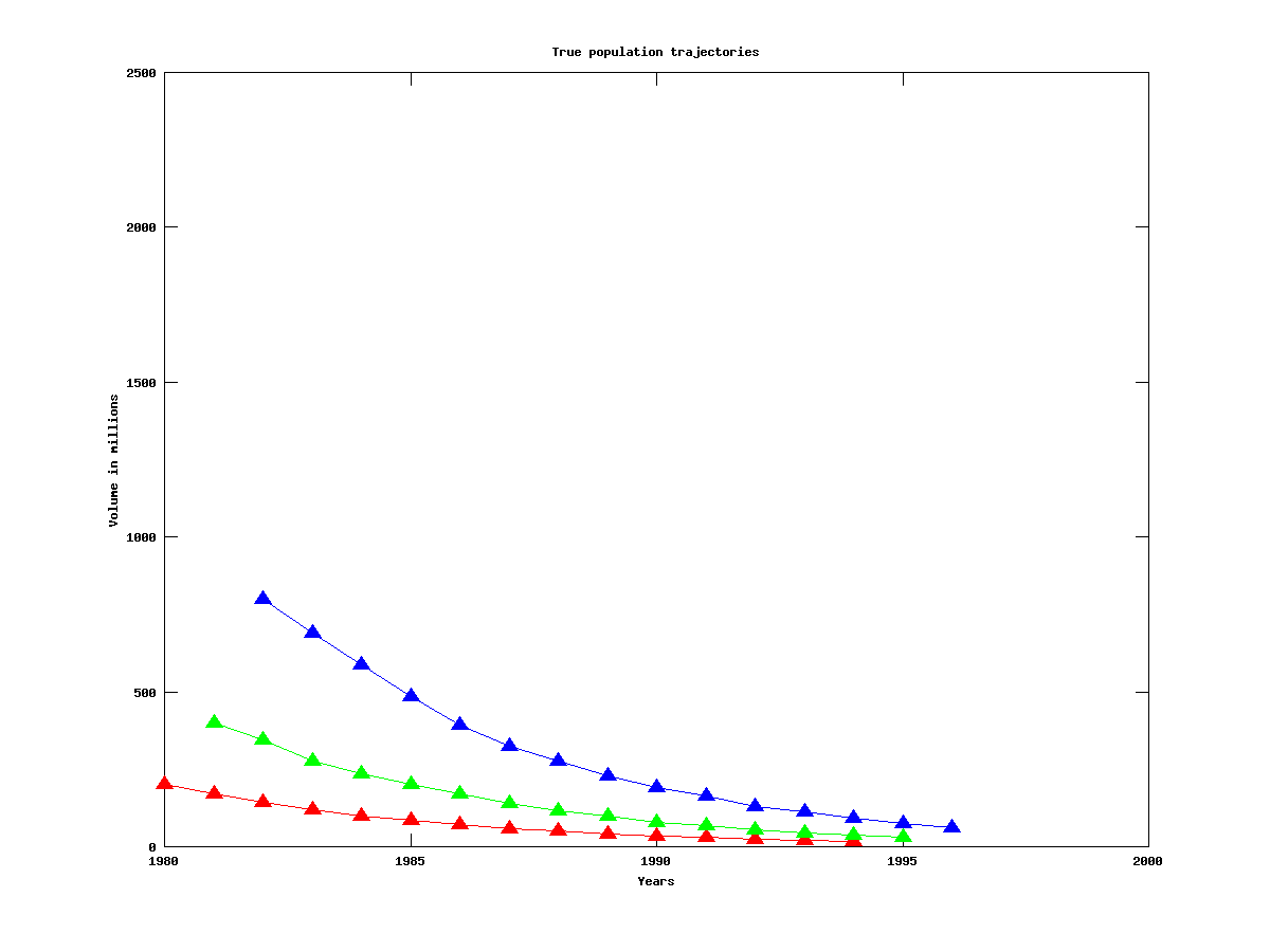
In other words, the recovered values are almost exactly the original values, which makes sense since the data was deterministic. The real population trajectories are shown in the figure below, with a different color for each cohort. (The recovered trajectories are almost identical, and are not shown.)

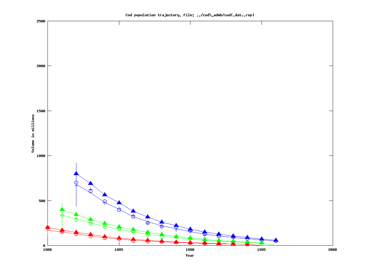
Instead of having deterministic data, let us set s to 0.05, and randomly generate a dataset (datfile, parfile, stdfile – the pinfile from the zero-sigma files defined earlier can still be used). This is then, of course, only one possible realization. If we optimize the model, we get the results in the figure below.
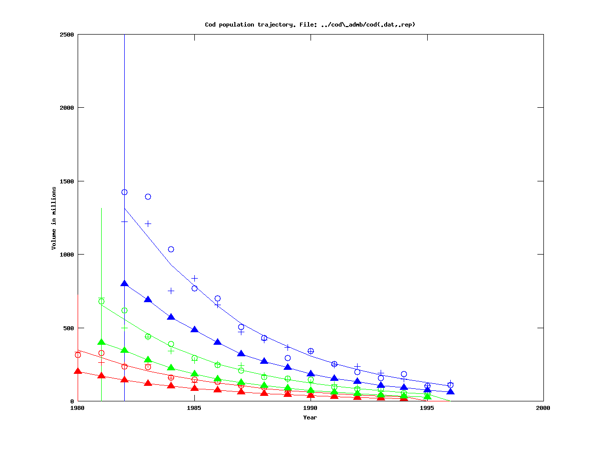
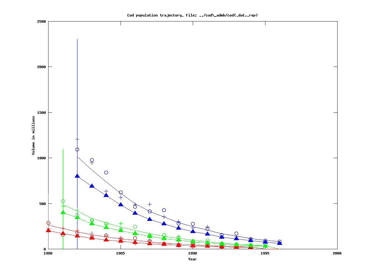
The curves with triangles are the true population trajectories. The plain curves are the computed trajectories, with a 95% confidence interval for the initial estimate marked as a vertical line. The plus sign and circles are survey observations from the first and second survey, respectively, DIVIDED BY the corresponding catchability. The colors of these observations correspond to the cohort colors.
Now, let us increase sigma to 0.1, and generate a new data set. (datfile, parfile, stdfile.) The results are given in the figure below:
The deviation between the computed and real trajectories is now slightly larger than for the prevoius case, as one might expect. However, the size of the confidence intervals has now grown dramatically. In addition, although the computed trajectories mathc the observations quite well, the observations do not match the true trajectories (especially for the blue curves), suggesting that the estimate of q is quite inaccurate. Indeed, from the stdfile we see that the estimated qs are about 0.3, as opposed to the true values of 0.5 for each survey.
Finally, let us try s = 0.15. (datfile, parfile, stdfile).
As one can see, the computed trajectories actually match the true curves better than they do for the previous case. This suggests that looking at only one realization per s-value is not enough in order to make inferences about the effect of s on the estimates. However, it can be noted that in this case the qs were estimated to be about 0.4, which is closer to the true values of 0.5, and this might explain why the fit is better.
Varying s in the data: Monte-Carlo experiments

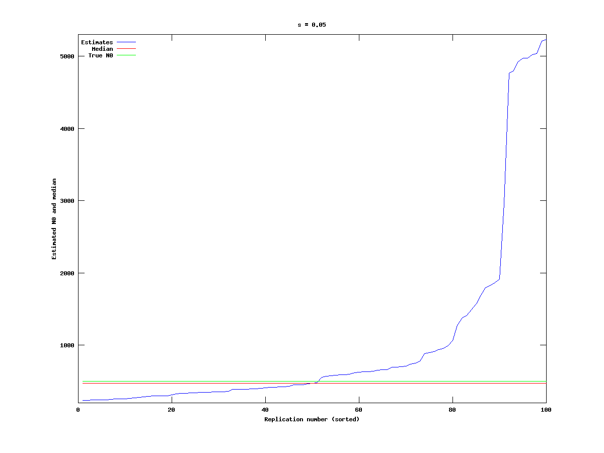
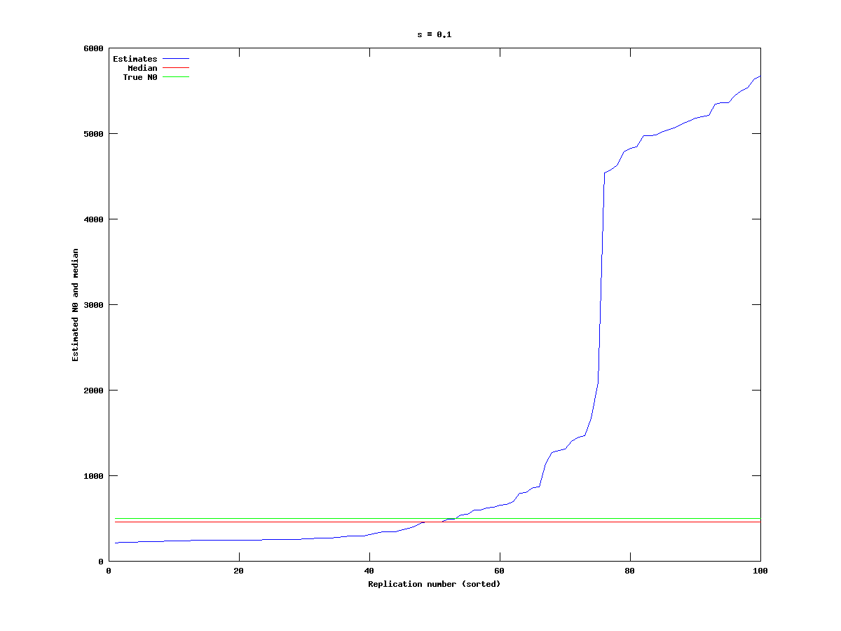
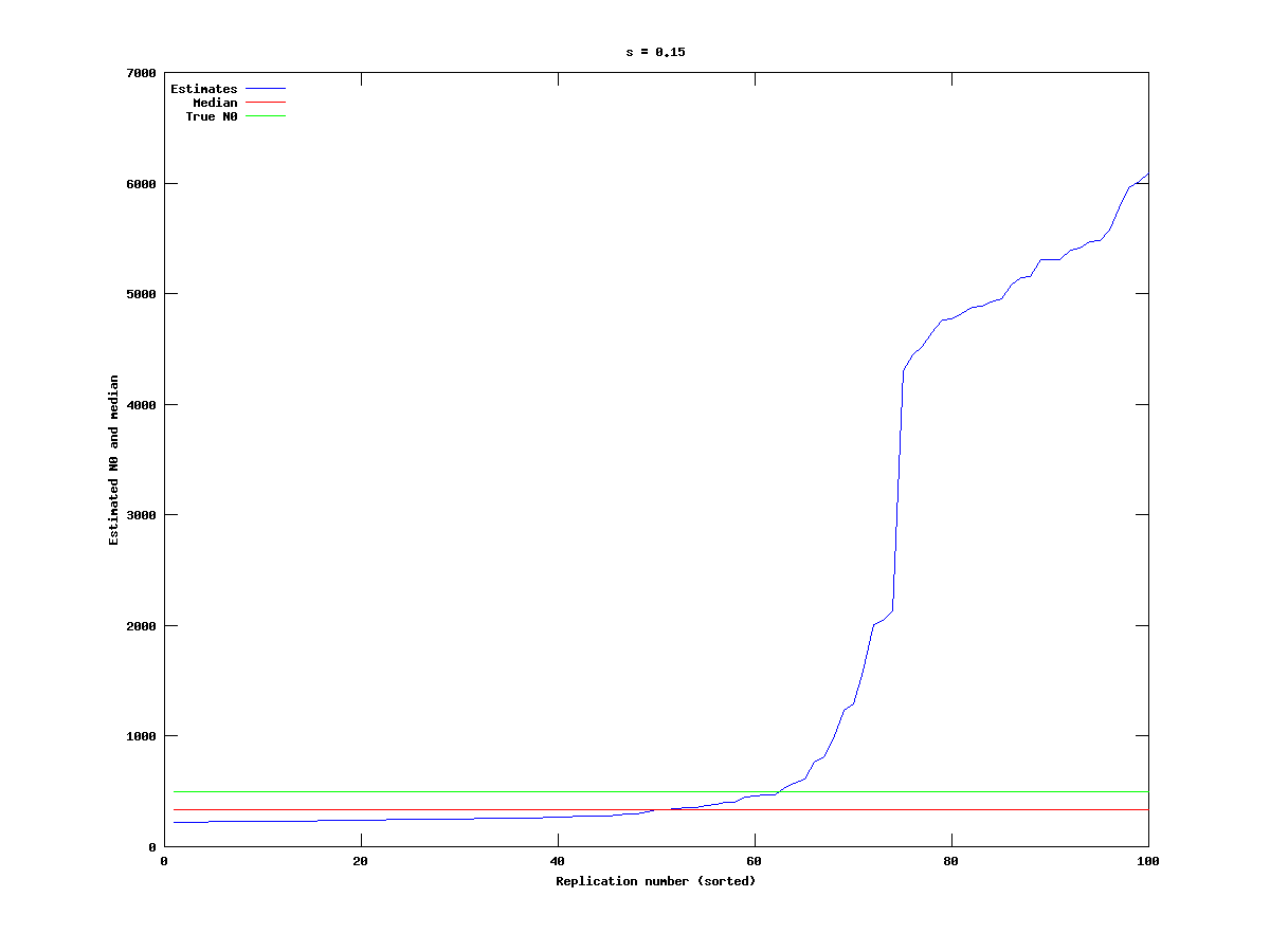
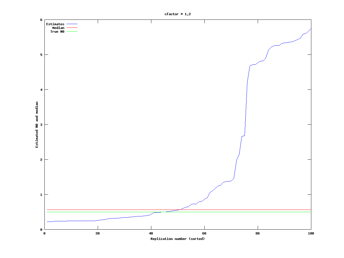
For the three choices of s (0.05, 0.1, 0.15) we generate data sets with one cohort which is followed for 15 years, with q = 0.5 and M = 0.15. The estimates for N0 vary a great deal, although the median is relatively stable, as shown in the figures below:
As one might expect, changing s has a significant effect on the number of experiments which produce estimates close to the true value, with a lower s-value giving better results.
Varying q in the data: Monte-Carlo experiments

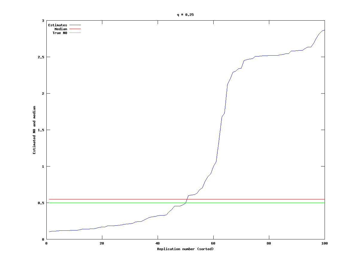
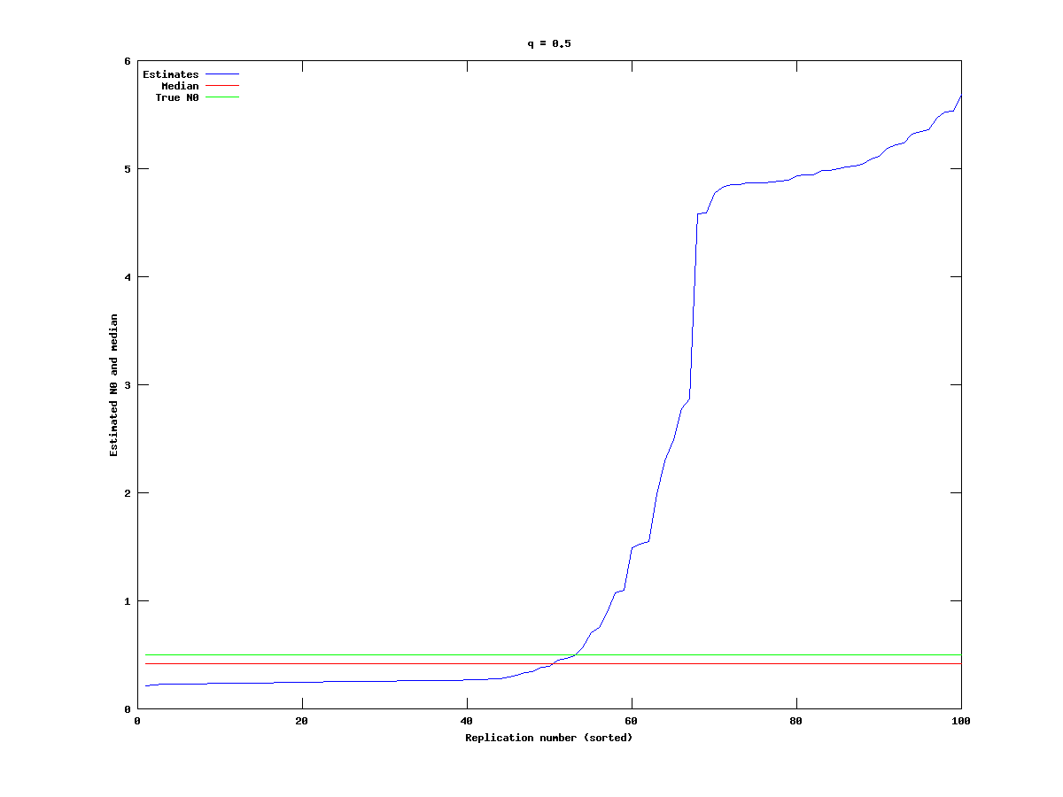
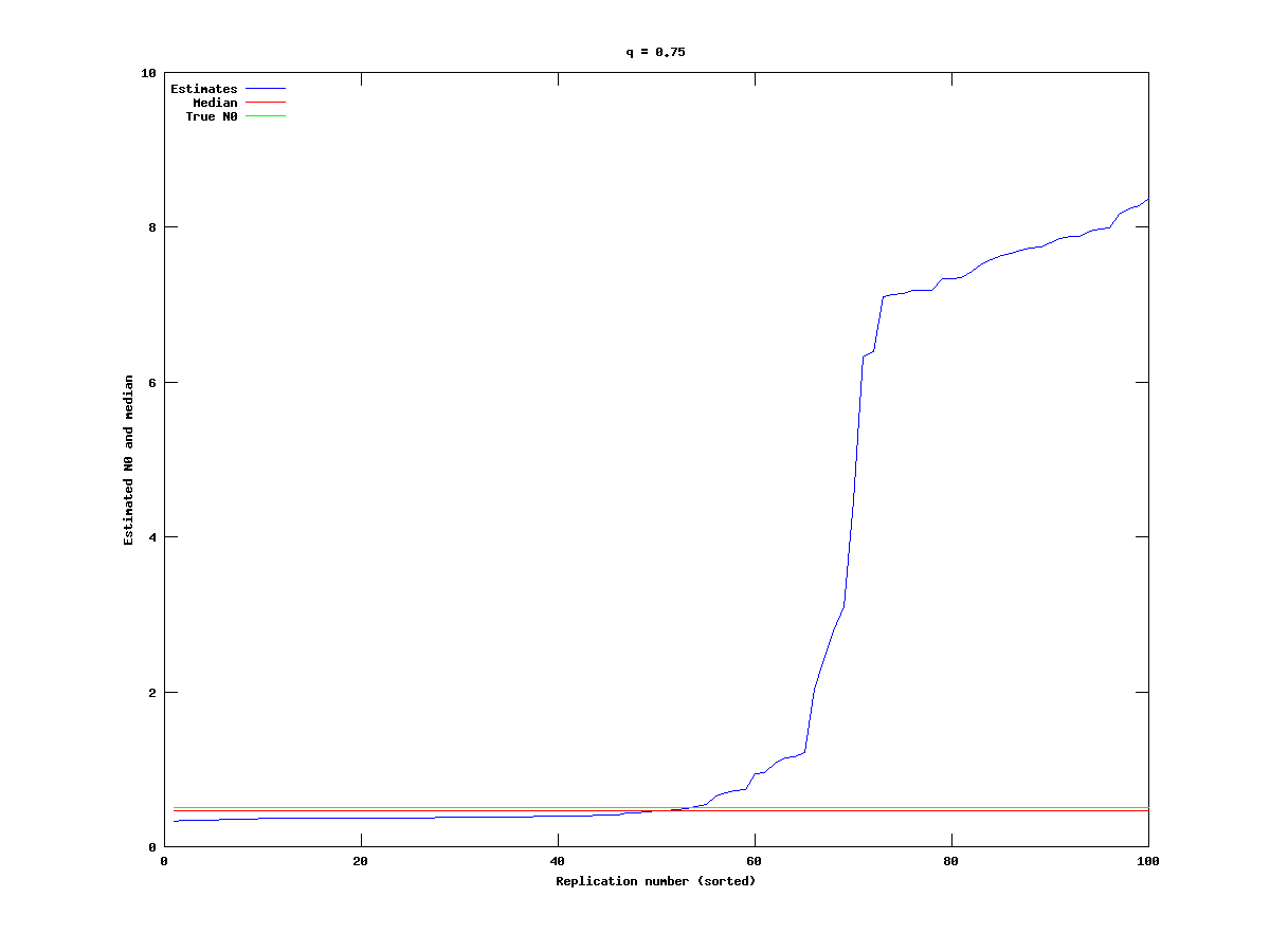
For the three choices of q (0.25, 0.5, 0.75) we generate data sets with one cohort which is followed for 15 years, with s = 0.1 and M = 0.15. As before, the estimates for N0 vary a great deal, although the median is relatively stable, as shown in the figures below:
As we can see, varying q has little effect, at least compared to varying s.
Varying M in the data: Monte-Carlo experiments

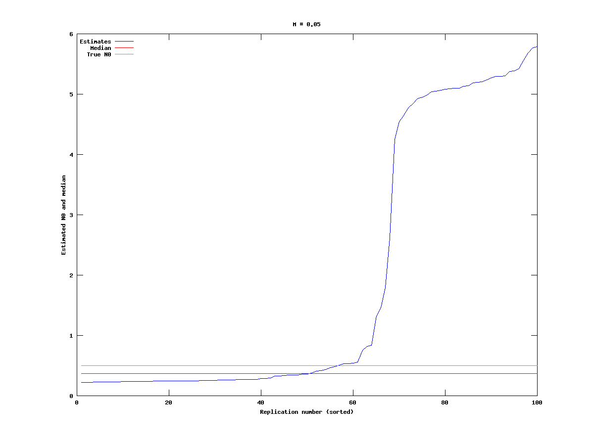
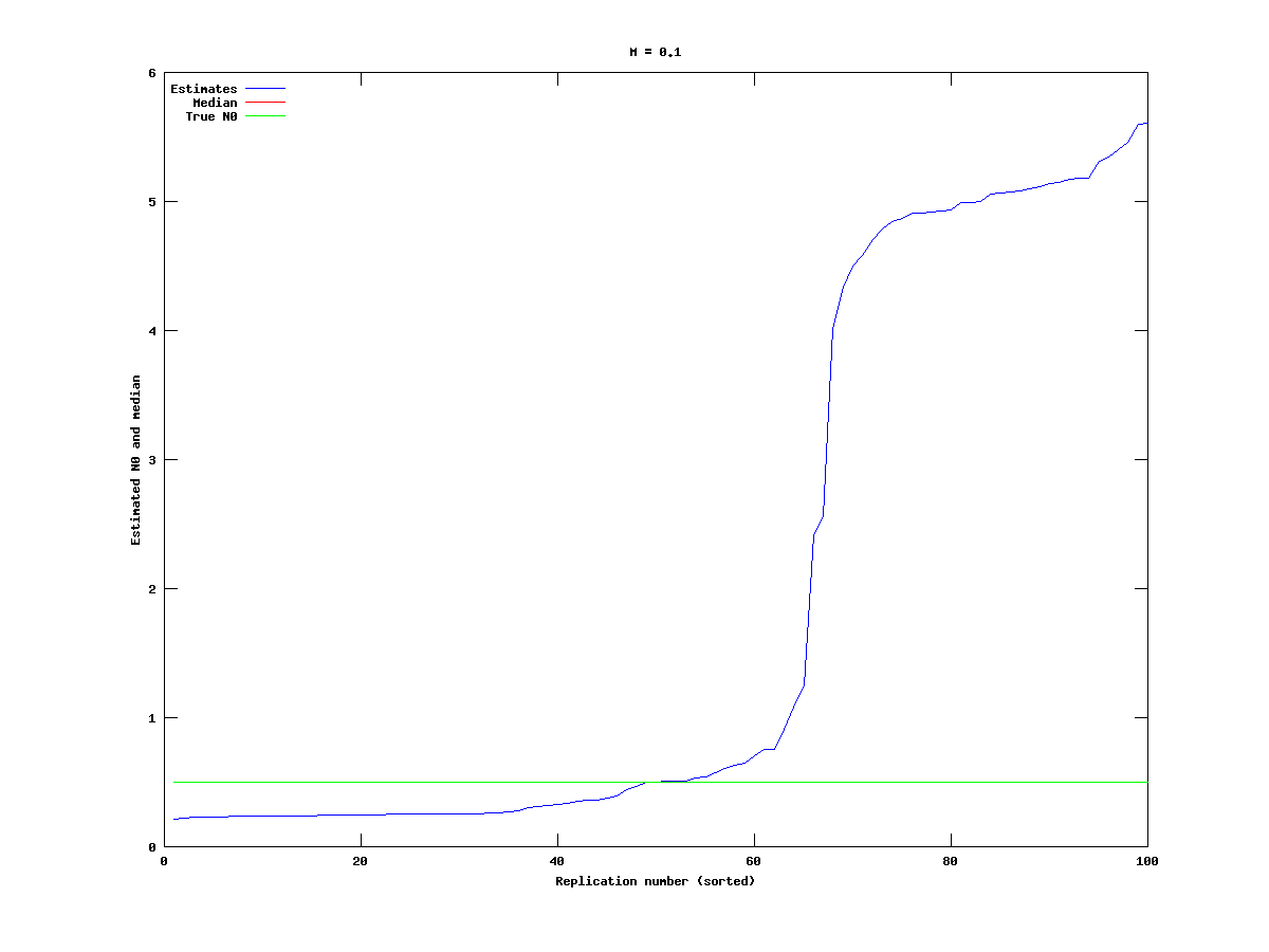
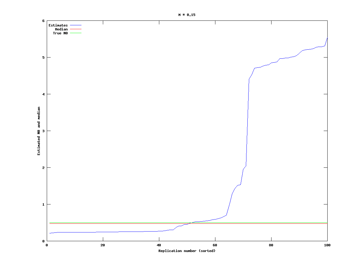
For the three choices of M (0.05, 0.1, 0.15) we generate data sets with one cohort which is followed for 15 years, with s = 0.1 and q = 0.5. As before, the estimates for N0 vary a great deal, but changing M does not seem to have an effect on the proportion of experiments which produce estimates for N0 that are much larger than the true value.
Varying cfactor in the data: Monte-Carlo experiments
For this set of experiments we vary the constant cfactor. It appears in the file generate_data on the line:
CC(i-1,j) = rand(1,1) * cfactor/n * N(i-1,j);
Here CC is the generated catch, n the number of years we follow the cohort, and N is the population level. What this line does is to set the catch for the year in question as fraction of the remaining stock multiplied with a uniformly distributed random variable. Increasing cfactor will therefore increase the catch.

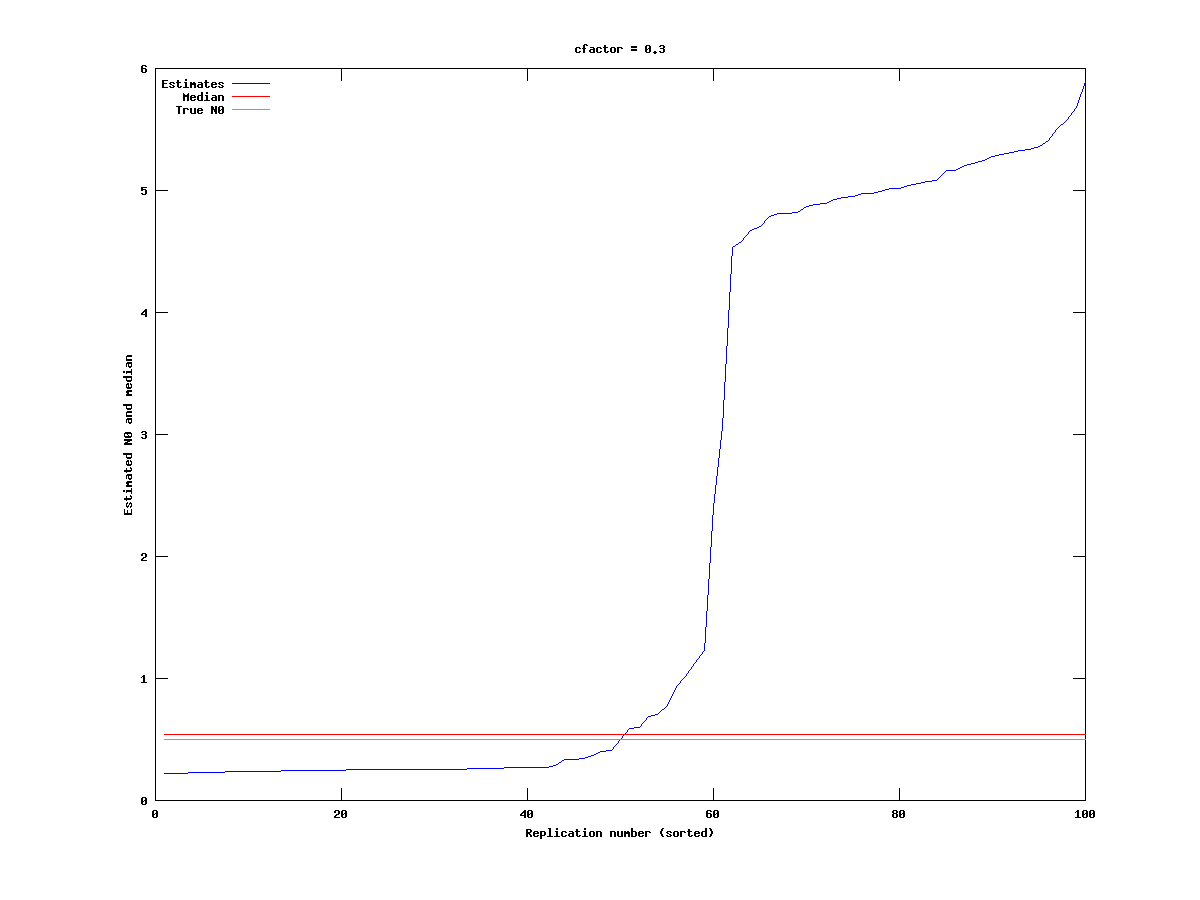
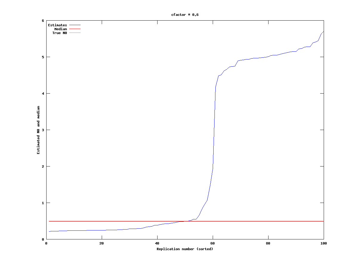
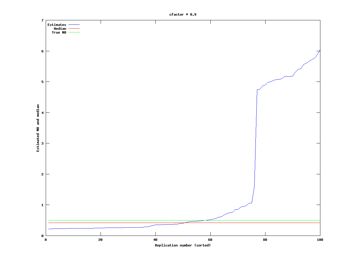
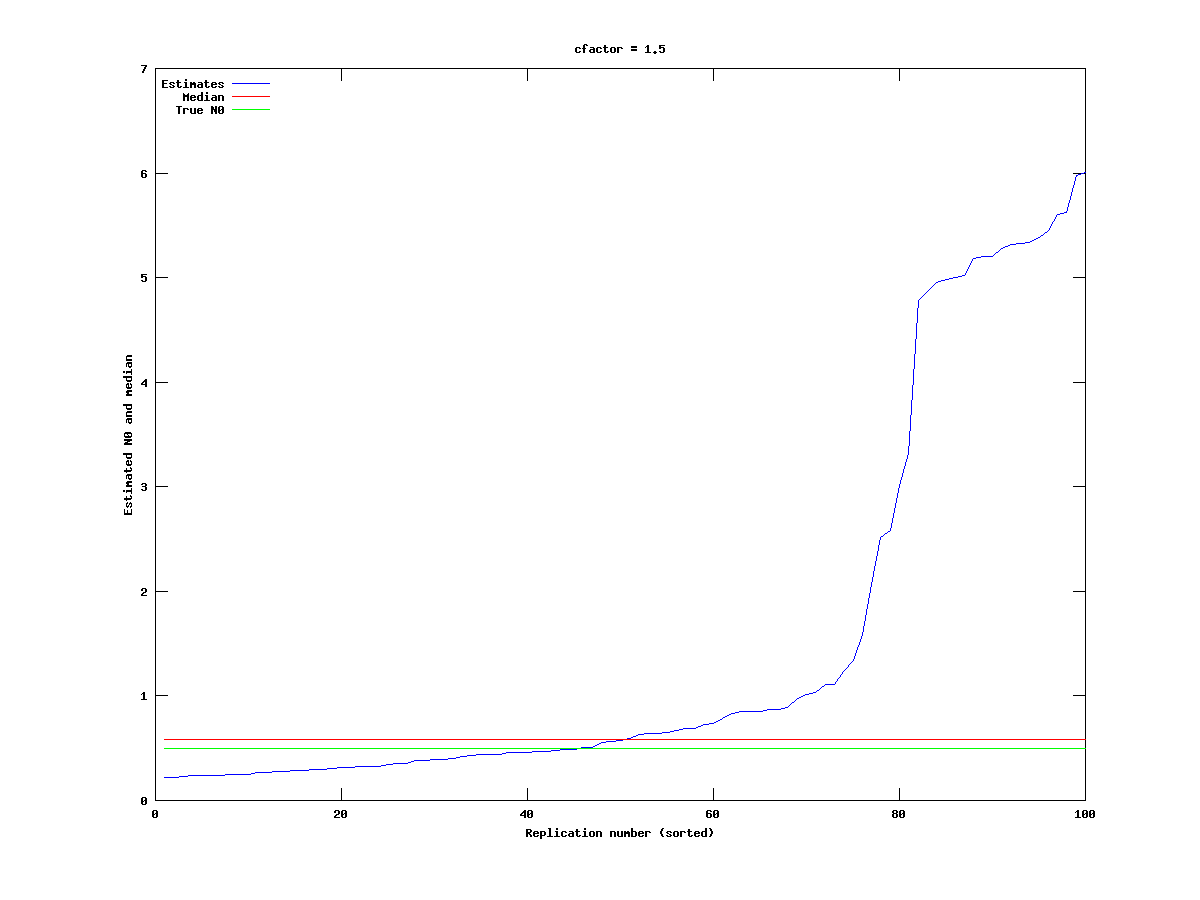
We test for five different values of cfactor (0.3, 0.6, 0.9, 1.2, 1.5). The results are shown in the following plots:
It appears to be the case that the N0 estimates become more stable as the catch increases, with the cfactor = 1.2 being a slight exception.
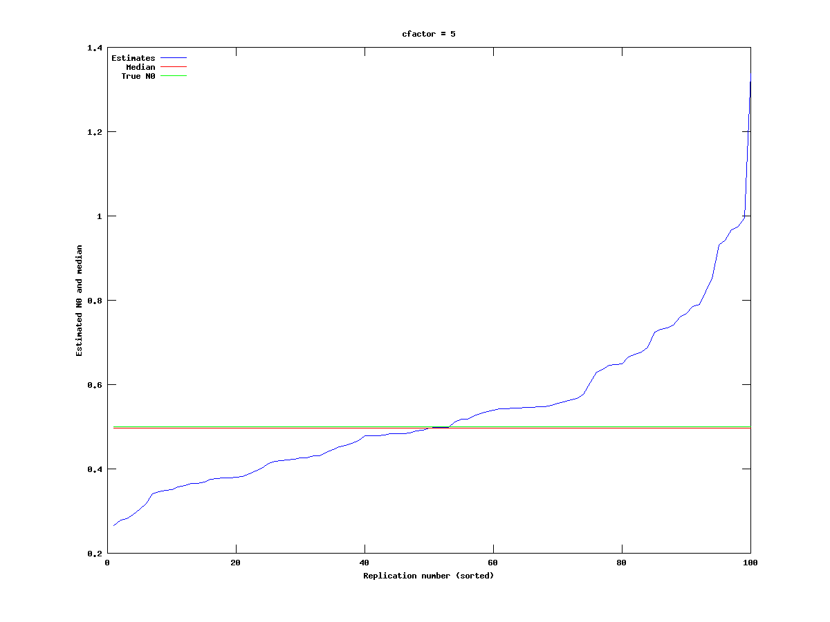
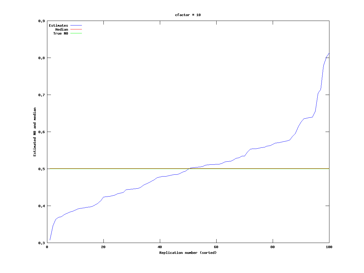
We therefore test two relatively large values, cfactor = 5 and 10. The results are given below:
As we can see, the estimates are now very consistent, but the case case cfactor = 10 corresponds to the cohort reaching almost zero level very quickly, (the order of 2-3 years), whereas cfactor = 5 allows the cohort to have reasonably large levels for about 7 years.

