Table of Contents
ADMAR-ADMB Framework
Simple Model
The ADMB framework is first tested on cod (Gadus morhua) data. In the first step, we start with a simple model [1] and an objective function [2], which is the log-likelihood function:
| Ni,t | = | (Ni,t-1-Ci,t-1)e-M | [1] |
|---|---|---|---|
| f(Ni,0,qk,s,M) | = | sumi,t,k{-(2s2)-1[ln(Ii,t,k)-ln(qkNi,t)]2-ln(s)} | [2] |
| Parameter | Description | Dimension |
|---|---|---|
| Ni,t | Number of indivduals in cohort i, at age t | m-by-(maxage+1) |
| M | Natural mortality | Scalar |
| Ci,t | Catch of indivduals in cohort i, at age t | m-by-(maxage+1) |
| Ii,t,k | Survey index for cohort i, at age t, by survey k | At most m-by-(maxage+1)-by-num_surveys |
| s | Standard deviation for I | Scalar |
| qk | Catchability of survey k | 1-by-num_surveys |
The number of cohorts and the number of surveys is determined by the input data. The free variables of the likelihood function are the m initial cohort sizes Ni,0 as well as qk, s and M.
Assumptions
The statistical assumption we make is that the survey data is log-normally distributed, that is: ln(Ii,t,k) ~ N(ln(qkNi,t),s2)
Implementation and Coding
We implement this as an ADMB template file:
- cod.tpl
// File: herring.tpl.
// Nedstrippet versjon til bruk ifm torsk på HI, 2010.
//
// Opprinnelig:
// Date: 29.09.02
// Author: Hans Julius Skaug (skaug@imr.no)
//
// Description: ADMB implementation of Sigurd's herring assessment.
//


DATA_SECTION

  // Fixed parameters in the model
  init_int 	m			// Number of cohorts

  !! cout << "Number of cohorts: " << m << endl;

  // Starting and ending year of cohort observation. Cohort is born in the
  // starting year.
  init_vector n_start_year(1,m)
  init_vector n_end_year(1,m)

  // Keep track of largest index of each cohort (it is not
  // a given that cohorts are followed for the same amount of years)
  // note that this index starts at zero
  vector n_largest_year_index(1,m)
  !! n_largest_year_index = n_end_year - n_start_year;
  !! cout << "n_largest_year_index " << n_largest_year_index << endl;

  // MATRIX WITH CATCH DATA, one cohort per row, one year per column
  // NOTE: The size of C is such that catch in the last year
  // (which won't be used for any computation) MUST be present!!
  // Setting it to zero is fine
  init_matrix C(1,m,0,n_largest_year_index)

  // Survey data
  init_int 	n_surv			// Number surveys

  !! cout << "Number of surveys: " << n_surv << endl;

  init_int 	n_I			// Number survey indices
  init_matrix I(1,n_I,1,4)		// "cohort","age","survey","I"
  // end of survey data

  // Number of calendar years our model spans. Computed from start and end years in data.
  int n_span
  !! n_span = max(n_end_year) - min(n_start_year) + 1;

  !! cout << "n_span = max(n_end_year) - min(n_start_year) + 1 = " << n_span << endl;
  !! cout << "Ignoring survey data for which there is no catch data!" << endl;


PARAMETER_SECTION

  // Recruitement
  init_bounded_vector   N0(1,m,0.01,10000);

  // Population trajectory, one cohort per row, one year per column.
  // (Entry i,j is year j in the life span of cohort i, which is calendar year
  // n_start_year(i)+j.) The width corresponds to the largest
  // life span we follow, so not all columns will be used unless all spans are the same.
  matrix 		N(1,m,0,n_span-1)

  // Catchability (survey specific)
  init_bounded_vector 	q(1,n_surv,.05,1.0)
  // Single q, from meeting with Sam 19Apr2010
  // init_bounded_number q0(.05,1.0)
  init_bounded_number 	logs(-5,3)		// Log standard deviation of survey errors
  number 	s				// Standard deviation of survey errors
  init_bounded_number   M(0,.5)                 // Mortality


  number tmp

  objective_function_value l


PRELIMINARY_CALCS_SECTION


GLOBALS_SECTION

  // Helper function to keep population nonnegative
  #include <fvar.hpp>
  dvariable posfun(_CONST dvariable&x,const double eps)
  {
    if (x>=eps)
    {
      return x;
    }
    else
    {
      dvariable y=1.0-x/eps;
      return eps*(1./(1.+y+y*y));
    }
  }

// Removed by LF 12032010
// #include <df1b2fun.h>

  //#include <df1b2loc.h>


PROCEDURE_SECTION

  int i,j;

  s= exp(logs);

  // initialize likelihood value
  l = 0;


  // Initialize N
  for(i=1;i<=(int) m;i++)
    N(i,0) = N0(i);


  // Compute population trajectory, note use of helper function posfun
  for(i=1;i<=m;i++) {
    for(j=1;j<=(int) n_end_year(i)-n_start_year(i);j++) {

      N(i,j) = posfun(N(i,j-1)-C(i,j-1),.01)*exp(-M);

    }
  }


  // Likelihood contributions from surveys
  for(i=1;i<=(int) n_I;i++)
  {
    // NEW --- LF, 19 Sept 2009
    // Only include survey index if it comes from a year where N actually has a meaningful value
    // That is, that it has been recursively computed
    if (  I(i,2) <= n_largest_year_index(I(i,1))  ) {
      tmp = (log(I(i,4))  - log(q(I(i,3)) *N(I(i,1),I(i,2)))) /s;
      // Single q, from meeting with Sam 19Apr2010
      // tmp = (log(I(i,4))  - log(q0 *N(I(i,1),I(i,2)))) /s;

      l += -.5*tmp*tmp - logs;
    }
  }

  // Reverse objective function sign since ADMB does minimization
  l *= -1;

  cout << setprecision(4);


REPORT_SECTION
  report << setprecision(4);
  //cout << "l="<< l << " N0=" << N0 << " q="<< q << " M=" << M  << " s=" << s << endl;

  report << N << endl;
TOP_OF_MAIN_SECTION
  arrmblsize = 50000000L;
  gradient_structure::set_GRADSTACK_BUFFER_SIZE(1000000);
  gradient_structure::set_CMPDIF_BUFFER_SIZE(2000000);
  gradient_structure::set_MAX_NVAR_OFFSET(40205);
Preliminary Results
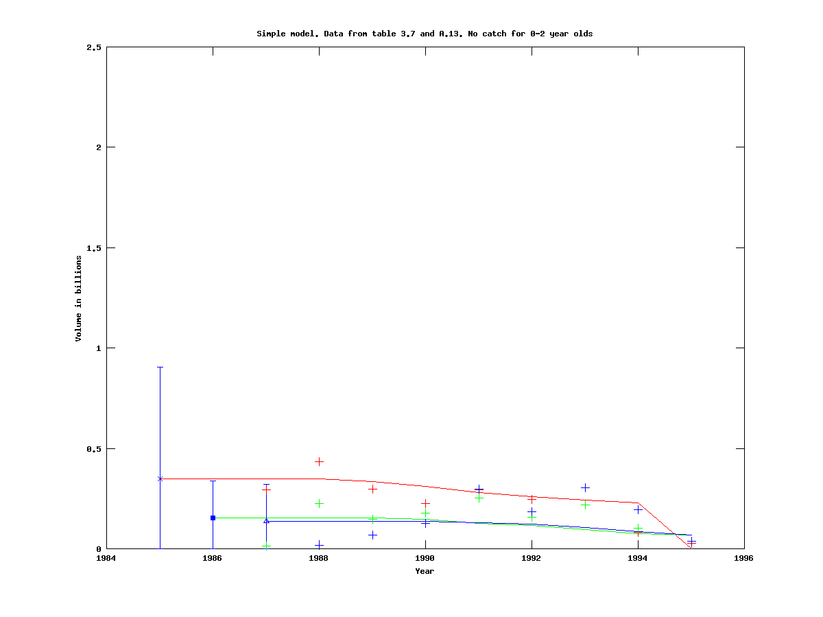
To test the initial model on real data, we use table 3.7 from the 2009 ICES AFWG report, with the catch for 0-2 year olds set to zero. The survey data is taken from table A.13 in the same document. (.dat-file) Population trajectories with 95% confidence intervals for the initial population size, for three cohorts starting in 1985, are given below. On the right are the contents of the file ending with .cor output by ADMB, which contains the estimates, standard deviations, and correlation matrix.
 |
|
Model with two mortality parameters
We now extend the model by introducing a latent variable, Mvec, which adjusts the mortality for age classes 7 and up.
| Ni,t | = | (Ni,t-1-Ci,t-1)e-M for t<7 | [1] |
|---|---|---|---|
| Ni,t | = | (Ni,t-1-Ci,t-1)e-(M+Mvec) for t >= 7 | |
| f(Ni,0,qk,s,M,Mvec) | = | sumi,t,k {-(2s2)-1[ln(Ii,t,k)-ln(qkNi,t)]2-ln(s)} -0.5 Mvec2 | [2] |

| g(Ni,0,qk,s,M) | Joint function [2] with Mvec as a constant, and Ni,0,qk,s,M as variables |
| h(Mvec) | Joint function [2] with Ni,0,qk,s,M as constants, and Mvec as the variable |
| Mvec | The maximum of h(Mvec) (for a given set of constants). |
| H(Mvec) | The Hessian of h(Mvec), evaluated at Mvec. |
Then the Laplace approximation (our objective function) is:
| g(Ni,0,qk,s,M) + 0.5 log( det( H(Mvec) ) ) | [3] |
|---|
In other words, for each function evaluation with the variables Ni,0,qk,s,M, as the input, an inner optimization problem must be solved to determine Mvec. This is done automatically by ADMB.
Assumptions
As for the simple model, the statistical assumption we make is that the survey data is log-normally distributed, that is: ln(Ii,t,k) ~ N(ln(qkNi,t),s2)
Implementation
The .tpl file then reads:

- cod.tpl
DATA_SECTION
  !! cout << "***************************************************************" << endl;
  !! cout << "* VERSION WITH SCALING, INPUT N0 WILL BE MULTIPLIED WITH 1000 *" << endl;
  !! cout << "***************************************************************" << endl;
  !! cout << endl;

  // Fixed parameters in the model
  init_int      m                       // Number of cohorts

  !! cout << "Number of cohorts: " << m << endl;

  // Starting and ending year of cohort observation. Cohort is born in the
  // starting year.
  init_vector n_start_year(1,m)
  init_vector n_end_year(1,m)

  // Keep track of largest index of each cohort (it is not
  // a given that cohorts are followed for the same amount of years)
  // note that this index starts at zero
  vector n_largest_year_index(1,m)
  !! n_largest_year_index = n_end_year - n_start_year;
  !! cout << "n_largest_year_index " << n_largest_year_index << endl;

  // MATRIX WITH CATCH DATA, one cohort per row, one year per column
  // NOTE: The size of C is such that catch in the last year
  // (which won't be used for any computation) MUST be present!!
  // Setting it to zero is fine
  init_matrix C(1,m,0,n_largest_year_index)

  // Survey data
  init_int      n_surv                  // Number surveys

  !! cout << "Number of surveys: " << n_surv << endl;

  init_int      n_I                     // Number survey indices
  init_matrix I(1,n_I,1,4)              // "cohort","age","survey","I"
  // end of survey data

  // Number of calendar years our model spans. Computed from start and end years in data.
  int n_span
  !! n_span = max(n_end_year) - min(n_start_year) + 1;

  !! cout << "n_span = max(n_end_year) - min(n_start_year) + 1 = " << n_span << endl;
  !! cout << "Ignoring survey data for which there is no catch data!" << endl;

PARAMETER_SECTION

  // Recruitement
  init_bounded_vector   N0(1,m,0.01,10000);

  // Population trajectory, one cohort per row, one year per column.
  // (Entry i,j is year j in the life span of cohort i, which is calendar year
  // n_start_year(i)+j.) The width corresponds to the largest
  // life span we follow, so not all columns will be used unless all spans are the same.
  matrix                N(1,m,0,n_span-1)

  // Catchability (survey specific)
  init_bounded_vector   q(1,n_surv,.05,1.0)
  // Single a, from meeting with Sam 19Apr2010
  //init_bounded_number q0(.05,1.0)
  init_bounded_number   logs(-5,3)              // Log standard deviation of survey errors
  number        s                               // Standard deviation of survey errors
  init_bounded_number   M(0,.5)                 // Mortality


  random_effects_vector Mvec(1,1)

  number tmp

  objective_function_value l


PRELIMINARY_CALCS_SECTION


GLOBALS_SECTION

  // Helper function to keep population nonnegative
  #include <fvar.hpp>
  dvariable posfun(_CONST dvariable&x,const double eps)
  {
    if (x>=eps)
    {
      return x;
    }
    else
    {
      dvariable y=1.0-x/eps;
      return eps*(1./(1.+y+y*y));
    }
  }

// Removed by LF 12032010
// #include <df1b2fun.h>

  //#include <df1b2loc.h>

PROCEDURE_SECTION

  int i,j;

  s= exp(logs);

  // initialize likelihood value
  l = 0;

  // Penalize random effects
  l -= 0.5 * norm2(Mvec);

  // Initialize N
  for(i=1;i<=(int) m;i++)
    N(i,0) = 1000*N0(i);


  // Compute population trajectory, note use of helper function posfun
  for(i=1;i<=m;i++) {
    for(j=1;j<=(int) n_end_year(i)-n_start_year(i);j++) {

      // NEW - mortality has two components, base mortality for age 0-6, and
      // a random effects correction term for ages 7 and up
      if (j>6) {
         N(i,j) = posfun(N(i,j-1)-C(i,j-1),.01)*exp(-M-Mvec(1));
      } else {
         N(i,j) = posfun(N(i,j-1)-C(i,j-1),.01)*exp(-M);
      }
    }
  }


  // Likelihood contributions from surveys
  for(i=1;i<=(int) n_I;i++)
  {
    // NEW --- LF, 19 Sept 2009
    // Only include survey index if it comes from a year where N actually has a meaningful value
    // That is, that it has been recursively computed
    if (  I(i,2) <= n_largest_year_index(I(i,1))  ) {
      tmp = (log(I(i,4))  - log(q(I(i,3)) *N(I(i,1),I(i,2)))) /s;
      // Single q, from meeting with Sam 19apr2010
      //  tmp = (log(I(i,4))  - log(q0 *N(I(i,1),I(i,2)))) /s;
        l += -.5*tmp*tmp - logs;
    }
  }

  // Reverse objective function sign since ADMB does minimization
  l *= -1;

  cout << setprecision(4);


REPORT_SECTION
  report << setprecision(4);
  //cout << "l="<< l << " N0=" << N0 << " q="<< q << " M=" << M  << " s=" << s << endl;

  report << N << endl;
TOP_OF_MAIN_SECTION
  arrmblsize = 50000000L;
  gradient_structure::set_GRADSTACK_BUFFER_SIZE(1000000);
  gradient_structure::set_CMPDIF_BUFFER_SIZE(2000000);
  gradient_structure::set_MAX_NVAR_OFFSET(40205);
The corresponding .pin file must have an initial value for the new parameter and may (if there are three cohorts and one survey) look like:
- cod.pin
# N0
1 1 1
# q
0.40
# log(s)
0.1
# M
0.2
# Mvec
0
Preliminary Results

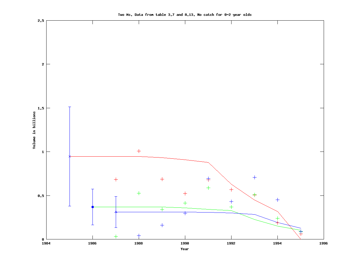
If we run the same experiment as for the simple model (.dat-file), we get the trajectories, 95% confidence intervals and output data below:
 |
|
The red curve in particular illustrates the effect of two different mortalities, since the slope changes significantly after seven years.
We now perform the same experiment, but instead of following three cohorts we follow 1, 2, 4 and 5 cohorts, to see how the output behaves.
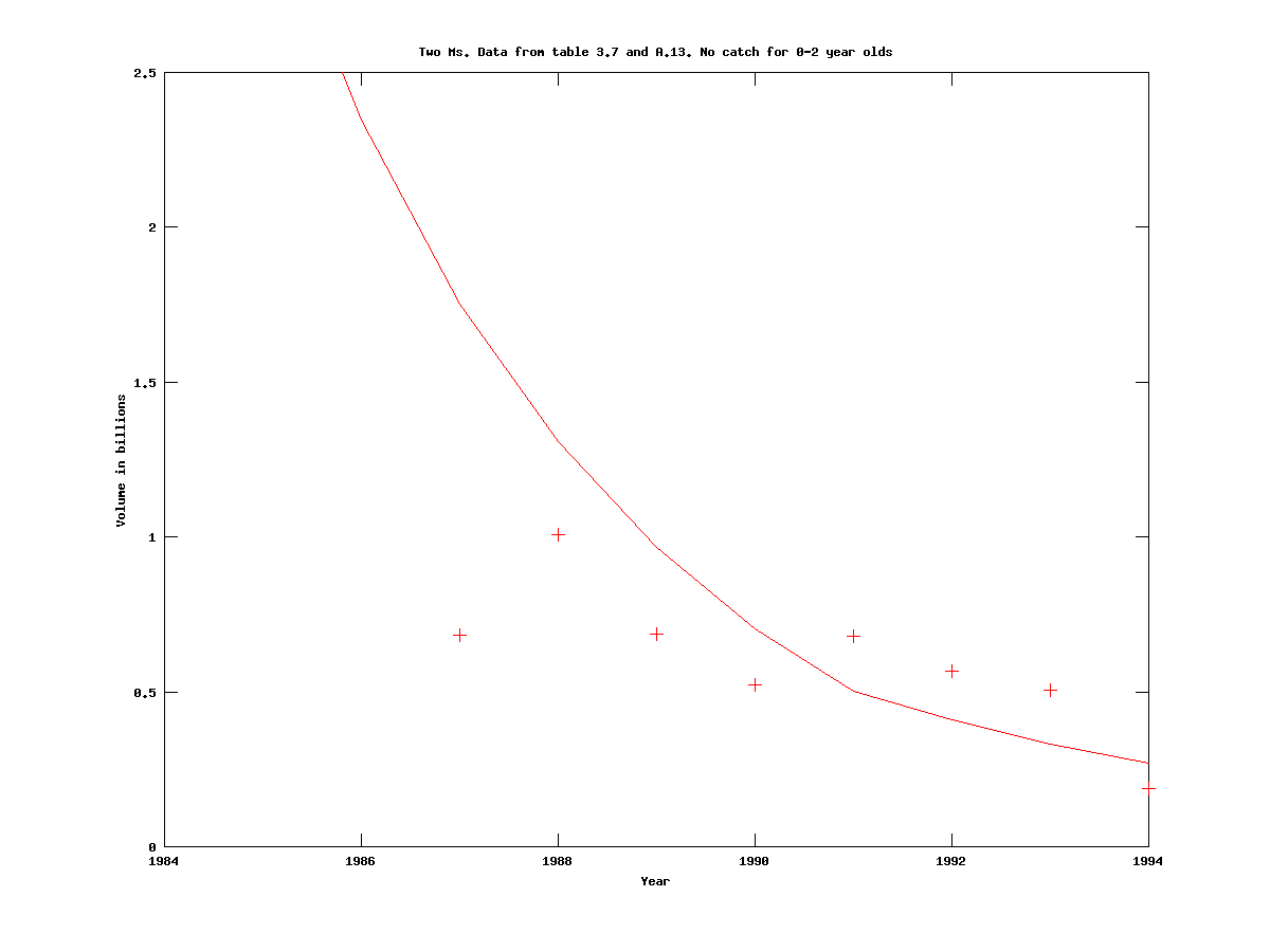
For the case of only one cohort (.dat-file), the trajectory is significantly different from the corresponding trajectory when estimating three cohorts, as can be seen in the figure below:
 |
|
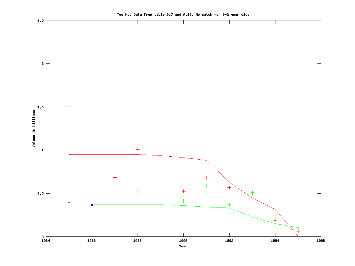
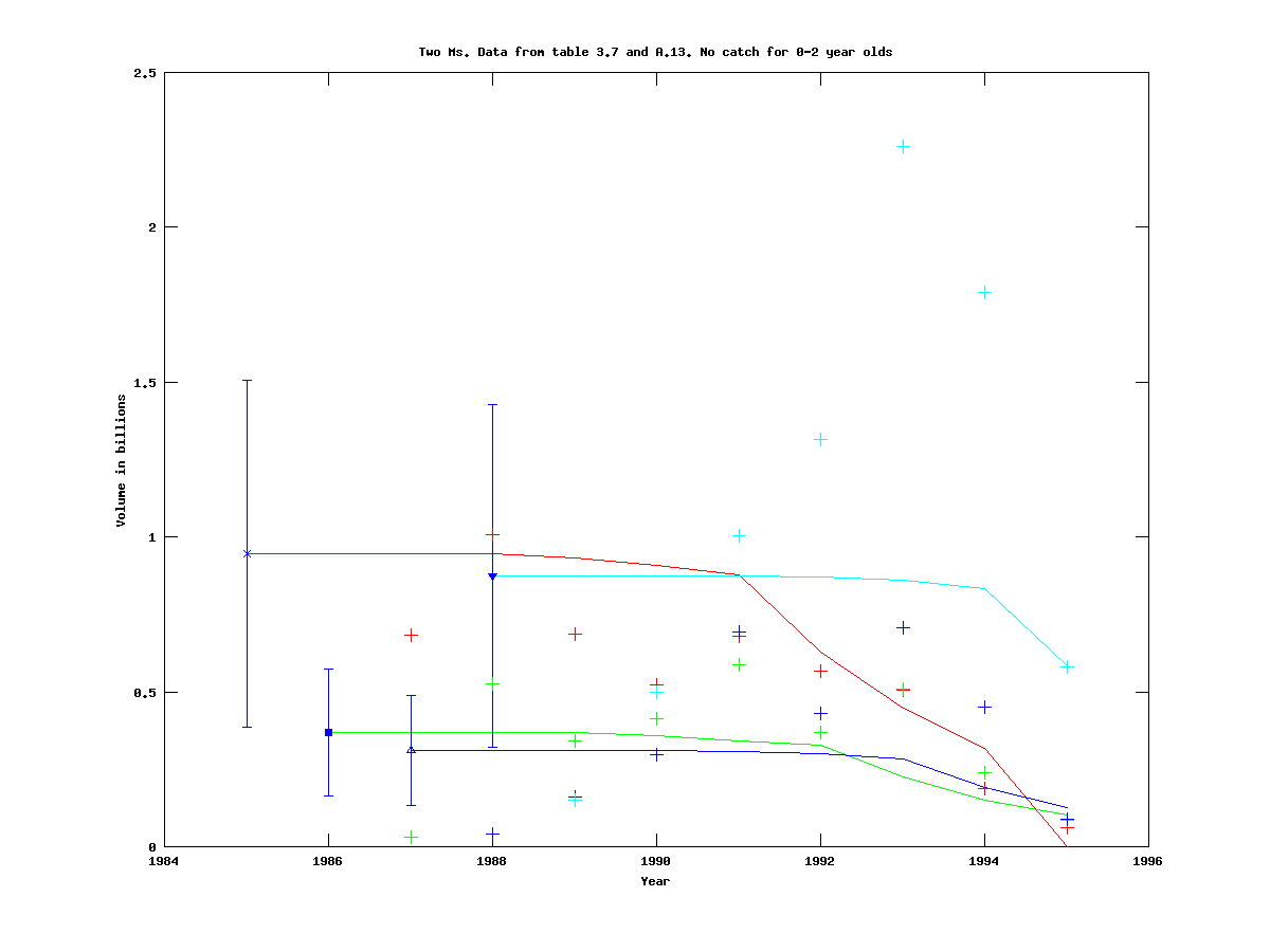
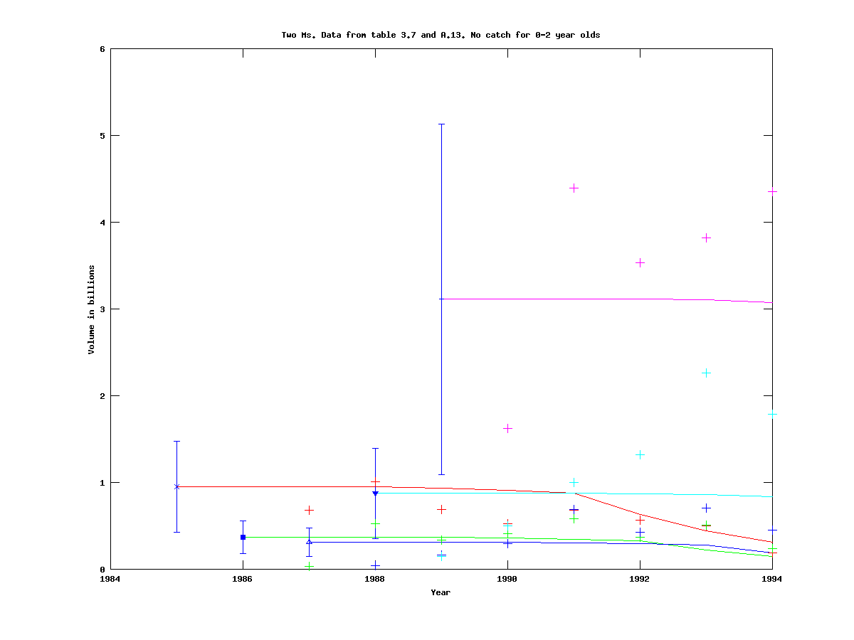
For 2, 4, and 5 cohorts, the trajectories do not change much, and are consistent with the case of three cohorts.
2 cohorts: (.dat-file)
 |
|
4 cohorts: (.dat-file)
 |
|
5 cohorts: (.dat-file)
 |
|
Note that the scale of the y-axis is different for the case of five cohorts.
Model with sigmoid function for catchability
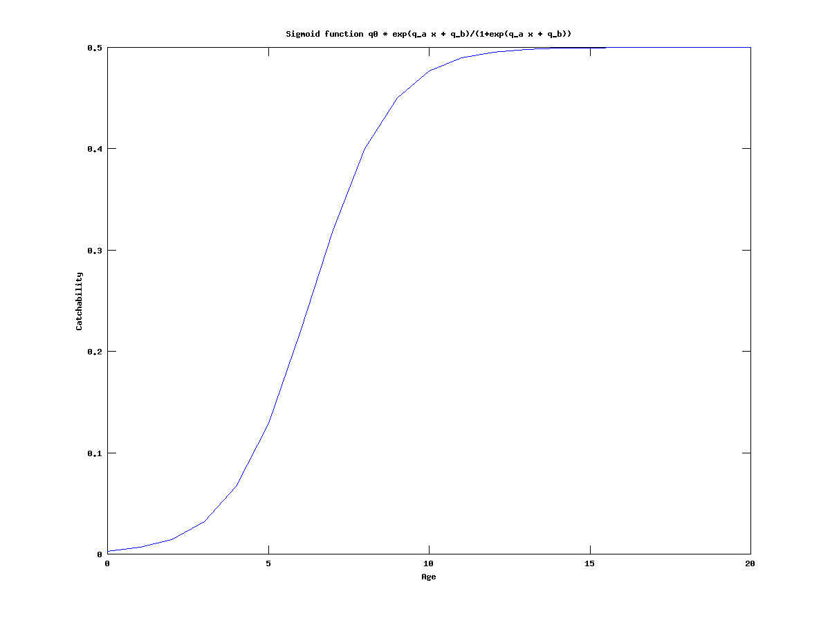
Since the estimates for the catchability q are very low, we try to model it with a sigmoid function. That is,
| Catchability | = | q0 exp(a x + b)/(1+exp(a x + b)) |
|---|
where the x represents the age of the cohort.

The model is implemented in this .tpl file. Note that the parameter structure is now different, so a .pin file for three cohorts should look like:
- cod.pin
# N0
1.000000  1.000000  1.000000

# q  alpha beta
0.60 1 1

# log(s)
0.1

# M
0.2
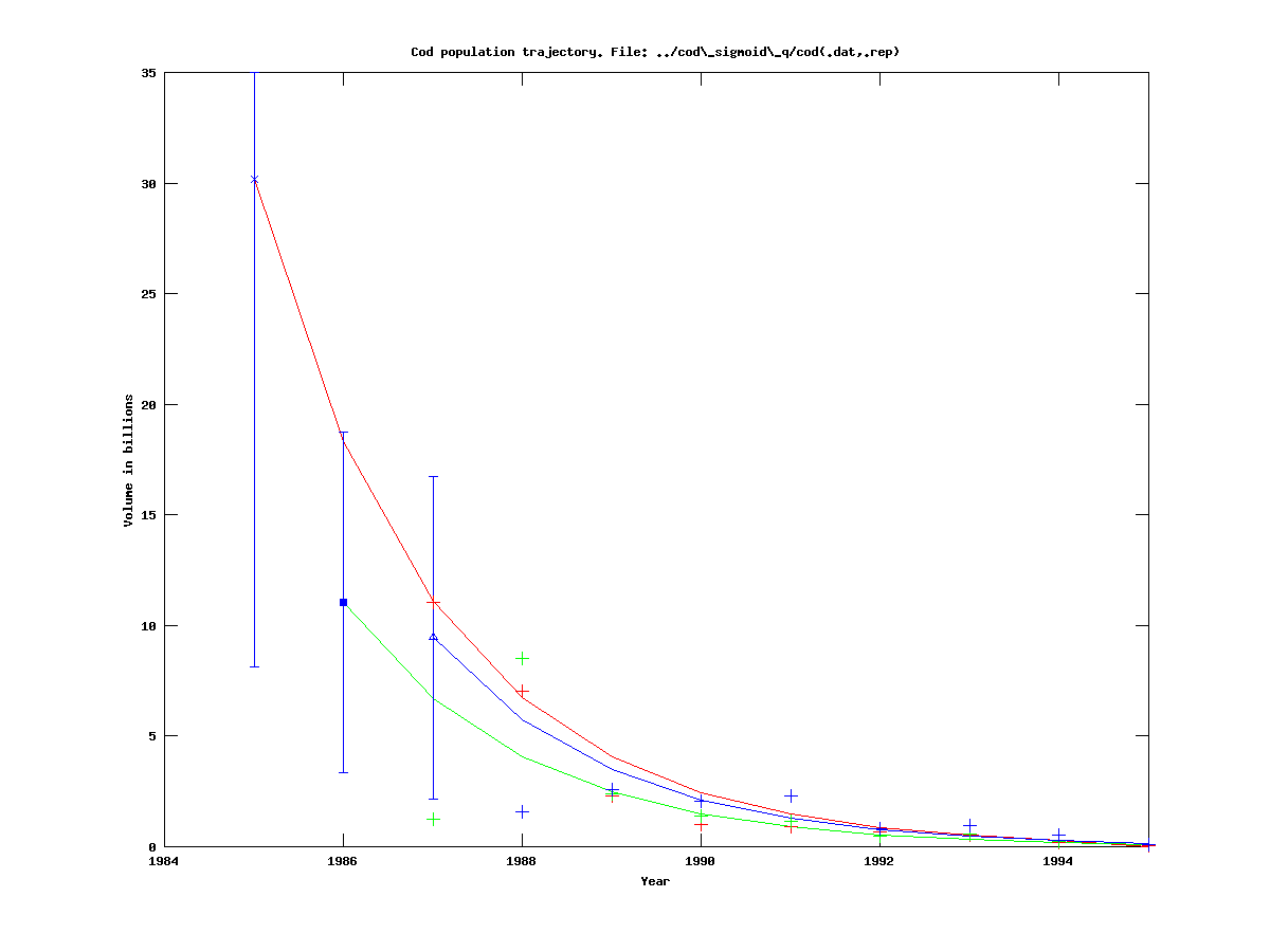
We run the model on the same dataset as before, and get:
 |
|
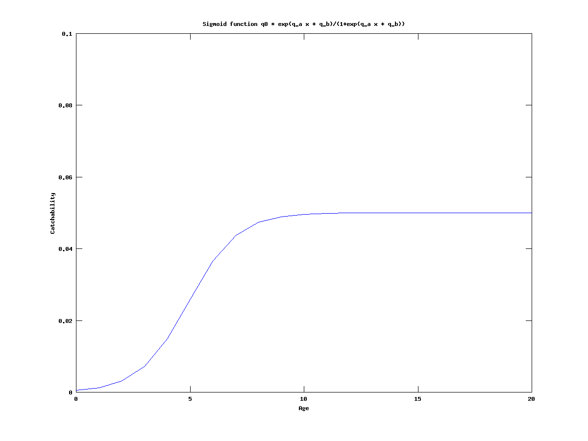 |
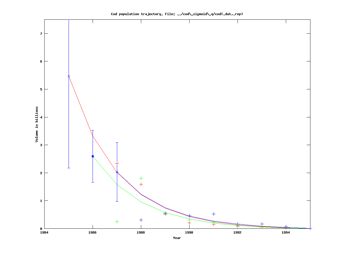
As one can see, the effective catchability is very low, due to the fact that q0 is at its lower bound of 0.05. Therefore we set the lower bound to be 0.5, (which requires editing of the .tpl file and recompilation), and then get:
 |
|
 |
As one can see, q is still at its lower bound, which seems to be the most important parameter for this model on this dataset.
Model with two separate catchabilities
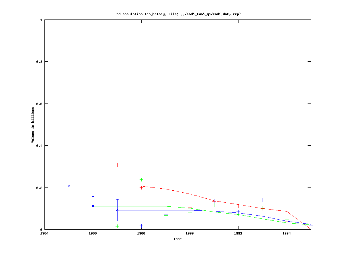
This model has two q variables for each survey, one which is applied to age groups 0-2, and one which is applied to age group 3 and up. It is implemented in this .tpl file. A .pin file for three cohorts may read:
- cod.pin
# N0
3.07 2.95 2.9
# q02
0.20
# q3plus
0.2
# log(s)
0.1
# M
0.1
We run it on the usual data set, and get:
 |
|
As one can see the catchability for the classes age 3 and up is larger than for 0-2 year olds, which is consistent with our expectations.
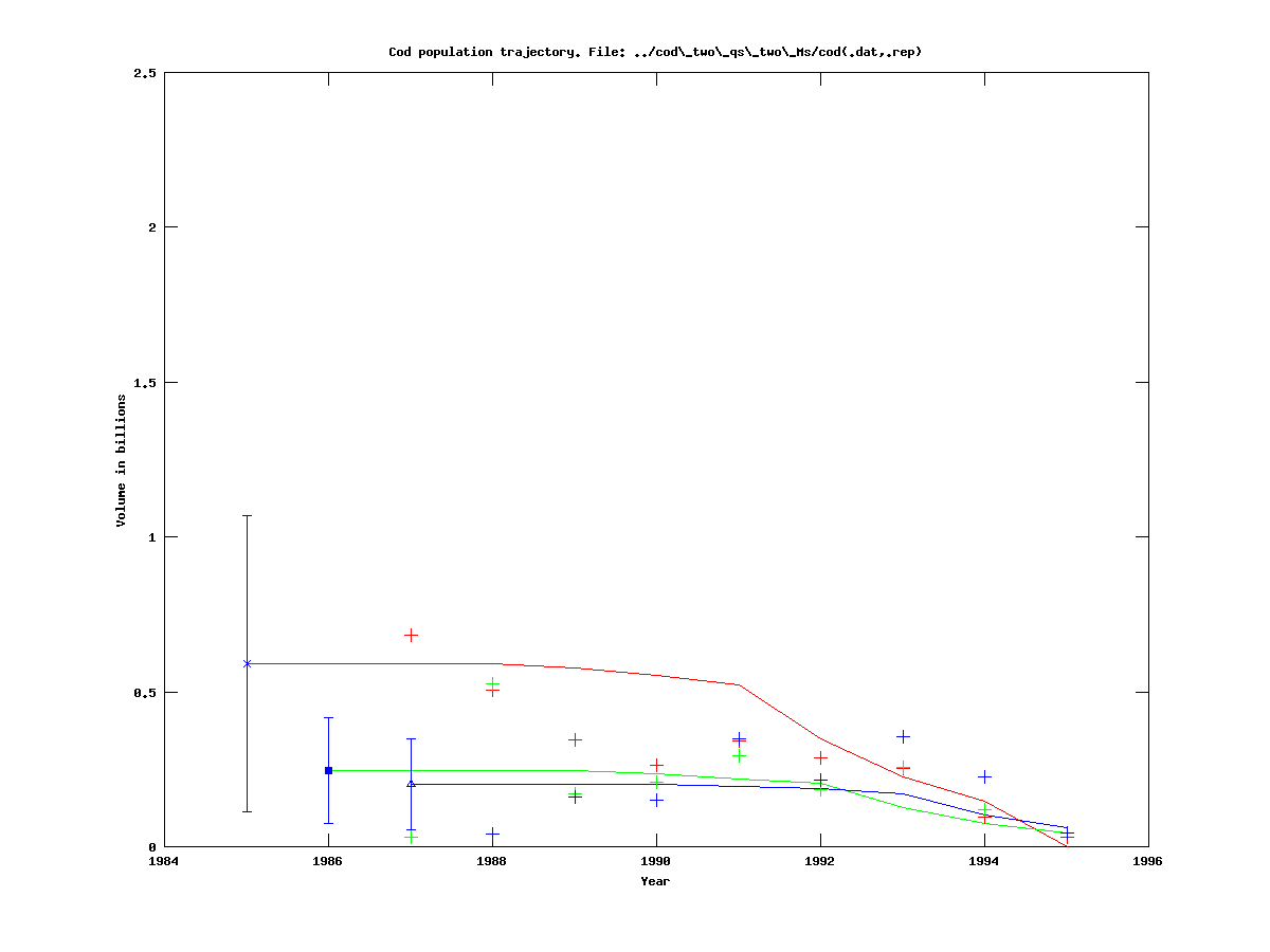
Model with two separate catchabilities and two mortalities
This model is a combination of the models with two Ms and two qs. The .tpl file can be found here. A .pin file should look like
- cod.pin
# N0
3.07 2.95 2.9
# q02
0.20
# q3plus
0.2
# log(s)
0.1
# M
0.1
# Mvec
0
We run it on the standard dataset and get:
 |
|
Note that the catchability for 0-2 year olds, q02, is at its lower bound of 0.05, whereas the catchability q3plus is not.
